Introduction

Simulators and mechanistic models are useful when the processes we care about contain latent variables that are difficult, or impossible, to observe directly. A biological example that originally motivated me to work in this area is understanding how bone morphogenetic protein (BMP) receptors and protein ligands interact to produce downstream gene expression.

At first glance, this might sound like a binding-affinity problem. Why not just use surface plasmon resonance (SPR)? The complication is that BMP signaling is not a simple one-to-one interaction. A signaling complex combines a protein ligand with two type I and two type II receptors, which then initiates a downstream intracellular signaling cascade.

We could imagine engineering fluorescent surface markers to determine whether receptors are bound, although multiplexing that experiment would already be nontrivial. Even then, measuring the steady state of receptor complex formation only tells us part of the story. Extracellular receptor binding is coupled to intracellular relays through SMAD proteins (and potentially other, unknown, mechanisms) that ultimately generate the downstream signal of interest.

So instead of observing every hidden biological quantity directly, we can ask a different question:

Which latent parameter settings could have generated the data we actually observed?

That brings us to simulation-based inference.

1. Why SBI? From simulations to latent parameters

Suppose we can simulate many possible realities using different latent parameter values $\theta$, which, in our BMP example, would contain the unknown “binding affinity” between proteins. If we have a faithful simulator of our process, we can generate simulated observations, $y$, compare them with reality, $y_o$, and favor the parameter values whose simulations resemble the observed data. So we can generate a dataset of parameter-simulation pairs $(\theta, y)$ and favor the $\theta$ that generates the $y$ closest to $y_o$.

In its simplest form, this is Approximate Bayesian Computation (ABC): simulate from the model, compare simulated and observed data, and retain parameter values that produce sufficiently similar outcomes. As the name suggests, this takes a Bayesian perspective where the parameters we drew came from a prior $\theta \sim p(\theta)$, which we use to draw samples from our simulator $y \sim p(y \mid \theta)$ - akin to sampling a likelihood (but we can’t actually evaluate the probabilities of the simulatoed samples) - and can condition on our observation to get samples from the posterior $p(\theta \mid y_o) \propto p(\theta) p(y_o \mid \theta)$. We don’t have the “inference objects” of the posterior or likelihood, but ABC methods essentially perform this process to return posterior samples. Also, as you can imagine, if we have a better prior (more information) then ABC is more-likely to simulate a result that looks like our observations.

On the other hand, modern simulation-based inference (SBI) methods can instead train neural networks to approximate an inference object: for example, the likelihood, posterior, or likelihood ratio. This can provide amortized inference, meaning that after training, the model can be reused for inference across many observations rather than repeating the full inference procedure from scratch.

That does not mean neural SBI is always the right tool. The ABC literature is deep, and individual scientific simulators often have quirks that make specialized inference procedures attractive. If the goal is extremely accurate inference for one particular observed dataset, amortization may not even be necessary. But when inference must be repeated across datasets, or when the learned inference object will be used for another task, amortization becomes especially useful.

One important example of that second case is experimental design.

2. Why experimental design? Choosing $\xi$ to learn more

In Bayesian optimal experimental design (BOED), the simulator has not only latent parameters $\theta$, but also a design variable $\xi$.

The design might represent a measurement time, experimental condition, dosage, sensor placement, or some other decision under the experimenter’s control. Changing $\xi$ changes what the simulator is likely to produce:

\[p(y \mid \theta, \xi).\]

The goal is therefore not merely to infer $\theta$. We would also like to choose a design $\xi$ that makes the resulting observation $y$ maximally informative about $\theta$.

A natural objective is the expected information gain (EIG):

\[\operatorname{EIG}(\xi) = \mathbb{E}_{p(\theta) p(y \mid \theta, \xi)} \left[ \log \frac{ p(\theta \mid y,\xi) }{ p(\theta) } \right].\]

Equivalently, we can view EIG as the expected reduction in uncertainty about the latent parameters:

\[\operatorname{EIG}(\xi) = \mathrm{H}[p(\theta)] - \mathbb{E}_{p(y\mid\xi)} \left[ \mathrm{H}[p(\theta\mid y,\xi)] \right].\]

An informative experiment is therefore one that is expected to move us from a broad prior toward a more concentrated posterior.

The traditional two-stage approach

A common strategy is roughly:

1. learn or approximate the inference object for candidate design(s), and
2. use Bayesian optimization to search for designs with high estimated information gain.

This works, but it can be expensive. Learning the inference object itself requires simulations, and Bayesian optimization then introduces an additional outer optimization loop. When individual simulator evaluations are costly (particle physics provides some extreme examples) the total computational burden can become substantial.

This motivates the main question behind our recent UAI 2026 work:

Can we learn the inference object and optimize the experimental design at the same time?

3. SBI-BOED: jointly learning the inference model and the design

For normalizing-flow-based SBI models, the answer turns out to be yes—with a few tricks.

Rather than first training an inference object and then running a separate design optimizer, SBI-BOED jointly optimizes the parameters of the learned likelihood and the experimental design. This allows one or multiple designs to be optimized during the same training procedure.

The key ingredient is a contrastive mutual-information objective based on InfoNCE. Because normalizing flows provide normalized density estimates, the learned likelihood can be inserted directly into an InfoNCE-style estimator of information gain. We then use the following equation in SBI-BOED

\[\operatorname{EIG}_i(\psi,\phi,L,\lambda) = \mathop{\mathbb{E}}\limits_{ \substack{ \xi_i\sim p_\psi(\xi) \\ \theta_0\sim p(\theta_0) \\ y_i\sim p(y_i\mid\theta_0,\xi_i) \\ \theta_{1:L}\sim p(\theta_{1:L}) } } \left[ \log \frac{ p_\phi(y_i\mid\theta_0,\xi_i)^{1+\lambda} }{ \displaystyle \frac{1}{1+L} \sum\nolimits_{\ell=0}^{L} p_\phi(y_i\mid\theta_\ell,\xi_i) } \right].\]

The $\lambda$ term regularizes likelihood fitting: increasing $\lambda$ places more emphasis on likelihood accuracy relative to the information-gain objective, while $\lambda = 0$ recovers the unregularized InfoNCE objective. In practice, this tradeoff also affects optimization stability, which we investigate in the paper.

In principle, this utility function gives us gradients with respect to both:

• the parameters of the inference model, and
• the experimental design $\xi$.

In practice, directly optimizing a single static design is surprisingly difficult.

Why optimize a distribution over designs?

Instead of representing the design as one point, we introduce a distribution over designs,

\[p_\psi(\xi).\]

Early in training, this distribution provides the conditional likelihood estimator with a range of nearby experimental designs. That variation gives the model information about which direction in design space becomes more informative.

As training proceeds, we temper the design distribution from broad to narrow. Early exploration helps identify promising regions of design space; later concentration allows the optimization to focus on the most informative designs.

The effect is fairly dramatic.

The important part is not simply that randomness helps optimization. The width of the design distribution changes the objective itself: a broad distribution averages information gain over many possible designs, whereas a narrow distribution increasingly concentrates the objective around a particular region. The tempering schedule therefore gradually transitions the model from exploration toward design optimization.

The harder test: non-differentiable scientific simulators

The motivating advantage of SBI-BOED is that the simulator itself does not need to be differentiable with respect to the design.

Some alternative approaches can propagate gradients through experimental designs when the simulator is differentiable, or when simulator outputs can be precomputed over a design grid. Those assumptions can be powerful, but they exclude many scientific simulators—including the BMP model that motivated this work. You can actually use reinforcement learning (RL) but that is very sample inefficient so have fun waiting for results before the heat death of the universe.

The BMP simulator therefore provides the more interesting test in our paper.

We find that SBI-BOED can discover useful experimental designs with substantially fewer simulator calls than the two-stage Bayesian-optimization approach while also producing strong downstream posterior inference. In particular, we evaluate posterior quality using the median distance between posterior predictive simulations and the observed data.

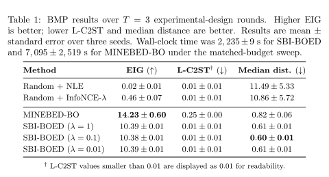
There is an interesting tradeoff here: Bayesian optimization can sometimes report a larger estimated EIG, while the designs obtained by SBI-BOED produce better downstream inference. Part of this discrepancy likely comes from finite-sample behavior of the InfoNCE bound and its approximation to the marginal likelihood; we discuss this tradeoff in more detail in the paper.

Taken together, the results suggest that jointly learning the inference object and experimental design can be both faster and more useful than repeatedly fitting inference models inside a separate optimization loop.

But this raises another question.

If SBI machinery can help us decide which experiment $\xi$ to run, can experimental-design machinery also help us decide which simulations $\theta$ to run?

4. Bridging back to SBI: active learning over $\theta$

So far, the direction of travel has been:

\[\text{SBI} \longrightarrow \text{experimental design}.\]

But the same information-theoretic machinery gives us a useful idea in the reverse direction.

Suppose the experimental design $\xi$ is fixed. Each simulator call now consists of choosing a latent parameter value $\theta$ and obtaining

\[y \sim p(y\mid\theta,\xi).\]

If simulator calls are expensive, sampling $\theta$ blindly from the prior may be wasteful. Some parameter values may produce observations that teach the likelihood model much more than others.

This turns ordinary SBI data collection into an active learning problem:

Which value of $\theta$ should we simulate next?

EPIG as an acquisition function for simulations

We use the same learned likelihood model to construct an expected predictive information gain (EPIG) score over candidate simulator parameters.

Rather than asking which experimental design is expected to reveal the most information about $\theta$, EPIG asks which simulator query $\theta$ is expected to be most informative for improving the predictive model.

The method uses MC-dropout to approximate epistemic uncertainty in the learned likelihood. Candidate $\theta$ values are compared against top-$K$ contrastive targets $\theta^\star$, and shared dropout particles are used to construct the joint predictive distribution.

The result is an acquisition rule over simulator parameters:

\[\theta_{\mathrm{next}} = \arg\max_\theta \operatorname{EPIG}(\theta).\]

We then simulate at $\theta_{\mathrm{next}}$, add the resulting $(\theta,y)$ pair to the training set, retrain, and repeat.

This is the part of the paper I find especially satisfying: the same information-based machinery works in both directions.

\[\boxed{ \text{choose }\xi \text{ to make experiments informative} } \qquad\longleftrightarrow\qquad \boxed{ \text{choose }\theta \text{ to make simulations informative} }\]

Active learning on Two Moons

We test this idea on the Two Moons benchmark and evaluate posterior calibration using the classifier two-sample test (C2ST).

Across active-learning rounds, EPIG-based acquisition generally improves over simply drawing new simulations from the prior across several choices of $K$ and $\lambda$.

Generally, beating “random” sampling from the prior resulted in better C2ST (1 is bad and 0.5 is best). $\ell$-C2ST is another metric for calibration (lower also better) that demonstrates that the $\lambda$ parameter is also important to tune for your problem and where hgiher sometimes is better - but depends on the simulator at hand.

One question we were not able to resolve completely is how $K$ and $\lambda$ should vary across active-learning problems. A decreasing $\lambda$ over successive acquisition rounds appears promising in our experiments, but the best schedule likely depends on the simulator and on how the learned likelihood evolves.

The broader point is that BOED and SBI need not be viewed as separate problems. Once both are expressed through information gain, ideas developed for choosing experiments can also help choose which simulations are worth paying for.

As a sanity check on the acquisition mechanism, we measured whether MC-dropout disagreement actually tracks likelihood error. Across active-learning rounds, dropout uncertainty is generally positively correlated with held-out deterministic NLL, suggesting that the stochastic likelihood particles identify regions where the model remains poorly learned.

Discussion

SBI-BOED combines simulation-based inference and Bayesian optimal experimental design into a single optimization procedure. By using an InfoNCE objective together with a tempered distribution over experimental designs, we can optimize informative designs without requiring the underlying simulator to be differentiable with respect to those designs.

The same perspective also leads naturally to active learning in ordinary SBI: when experimental conditions are fixed, the information objective can instead be used to prioritize which latent parameter values should be simulated.

This is the sense in which I think of the method as information bridging:

\[\text{inference} \longleftrightarrow \text{experimental design} \longleftrightarrow \text{active simulation acquisition}.\]

Code is available at LFIAX. Full paper is available here.

Future work includes extending these ideas to diffusion and flow-matching likelihood models, scaling to higher-dimensional scientific simulators, and understanding how the contrastive and active-learning hyperparameters should change as the simulation budget grows.

If you have a scientific simulator where these ideas might be useful, feel free to reach out via the email in my CV — I’m always happy to talk about potential applications or collaborations.